| 33 | Expressions and Their Structure |
We’ve now seen all sorts of things that exist in the Wolfram Language: lists, graphics, pure functions and much more. And now we’re ready to discuss a very fundamental fact about the Wolfram Language: that each of these things—and in fact everything the language deals with—is ultimately constructed in the same basic kind of way. Everything is what’s called a symbolic expression.
Symbolic expressions are a very general way to represent structure, potentially with meaning associated with that structure. f[x, y] is a simple example of a symbolic expression. On its own, this symbolic expression doesn’t have any particular meaning attached, and if you type it into the Wolfram Language, it’ll just come back unchanged.
f[x, y] is a symbolic expression with no particular meaning attached:
In[1]:=
Out[1]=
{x, y, z} is another symbolic expression. Internally, it’s List[x, y, z], but it’s displayed as {x, y, z}.
The symbolic expression List[x, y, z] displays as {x, y, z}:
In[2]:=
Out[2]=
Symbolic expressions are often nested:
In[3]:=
Out[3]=
FullForm shows you the internal form of any symbolic expression.
In[4]:=
Out[4]=
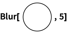
Graphics[Circle[{0, 0}]] is another symbolic expression, that just happens to display as a picture of a circle. FullForm shows its internal structure.
This symbolic expression displays as a circle:
In[5]:=
Out[5]=
FullForm shows its underlying symbolic expression structure:
In[6]:=
Out[6]=
Symbolic expressions often don’t just display in special ways, they actually evaluate to give results.
A symbolic expression that evaluates to give a result:
In[7]:=
Out[7]=
The elements of the list evaluate, but the list itself stays symbolic:
In[8]:=
Out[8]=
Here’s the symbolic expression structure of the list:
In[9]:=
Out[9]=
This is just a symbolic expression that happens to evaluate:
In[10]:=
Out[10]=

You could write it like this:
In[11]:=
Out[11]=

What are the ultimate building blocks of symbolic expressions? They’re called atoms (after the building blocks of physical materials). The main kinds of atoms are numbers, strings and symbols.
Things like x, y, f, Plus, Graphics and Table are all symbols. Every symbol has a unique name. Sometimes it’ll also have a meaning attached. Sometimes it’ll be associated with evaluation. Sometimes it’ll just be part of defining a structure that other functions can use. But it doesn’t have to have any of those things; it just has to have a name.
A crucial defining feature of the Wolfram Language is that it can handle symbols purely as symbols—“symbolically”—without them having to evaluate, say to numbers.
In the Wolfram Language, x can just be x, without having to evaluate to anything:
In[12]:=
Out[12]=
x does not evaluate, but the addition is still done, here according to the laws of algebra:
In[13]:=
Out[13]=
Given symbols like x, y and f, one can build up an infinite number of expressions from them. There’s f[x], and f[y], and f[x, y]. Then there’s f[f[x]] or f[x, f[x, y]], or, for that matter, x[x][y, f[x]] or whatever.
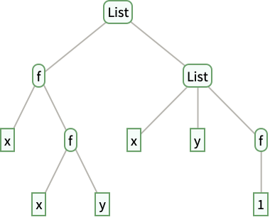
In general, each expression corresponds to a tree, whose ultimate “leaves” are atoms. You can show an expression as a tree using ExpressionTree.
An expression shown as a tree:
In[1435]:=
Out[1435]=
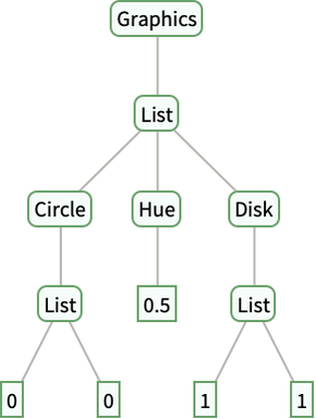
Here’s a graphics expression shown as a tree:
In[1436]:=
Out[1436]=
Because expressions ultimately have a very uniform structure, operations in the Wolfram Language operate in a very uniform way on them.
This is equivalent to {x, y, z}[[2]], which extracts the second element in a list:
In[16]:=
Out[16]=
Extracting parts works exactly the same way for this expression:
In[17]:=
Out[17]=
This extracts the circle from the graphics:
In[18]:=
Out[18]=
This goes on and extracts the coordinates of its center:
In[19]:=
Out[19]=
This works exactly the same:
In[20]:=
Out[20]=
In f[x, y], f is called the head of the expression. x and y are called arguments. The function Head extracts the head of an expression.
The head of a list is List:
In[21]:=
Out[21]=
Every part of an expression has a head, even its atoms.
The head of an integer is Integer:
In[22]:=
Out[22]=
The head of an approximate real number is Real:
In[23]:=
Out[23]=
The head of a string is String:
In[24]:=
Out[24]=
Even symbols have a head: Symbol.
In[25]:=
Out[25]=
In patterns, you can ask to match expressions with particular heads. _Integer represents any integer, _String any string and so on.
In[26]:=
Out[26]=
Named patterns can have specified heads too:
In[27]:=
Out[27]=
In using the Wolfram Language, most of the heads you’ll see are symbols. But there are important cases where there are more complicated heads. One such case is pure functions—where when you apply a pure function, the pure function appears as the head.
In[28]:=
Out[28]=
When you apply the pure function, it appears as a head:
In[29]:=
Out[29]=
As you become more sophisticated in Wolfram Language programming, you’ll encounter more and more examples of complicated heads. In fact, many functions that we’ve already discussed have operator forms where they appear as heads—and using them in this way leads to very powerful and elegant styles of programming.
Select appears as a head here:
In[30]:=
Out[30]=
In[31]:=
Out[31]=
All the basic structural operations that we have seen for lists work exactly the same for arbitrary expressions.
Length does not care what the head of an expression is; it just counts arguments:
In[32]:=
Out[32]=
/@ does not care about the head of an expression either; it just applies a function to the arguments:
In[33]:=
Out[33]=
Since there are lots of functions that generate lists, it’s often convenient to build up structures as lists even if eventually one needs to replace the lists with other functions.
@@ effectively replaces the head of the list with f:
In[34]:=
Out[34]=
This yields Plus[1, 1, 1, 1], which then evaluates:
In[35]:=
Out[35]=
This turns a list into a rule:
In[36]:=
Out[36]=
Here’s a simpler alternative, without the explicit pure function:
In[37]:=
Out[37]=
A surprisingly common situation is to have a list of lists, and to want to replace the inner lists with some function. It’s possible to do this with @@ and /@. But @@@ provides a convenient direct way to do it.
Replace the inner lists with f:
In[38]:=
Out[38]=
In[39]:=
Out[39]=
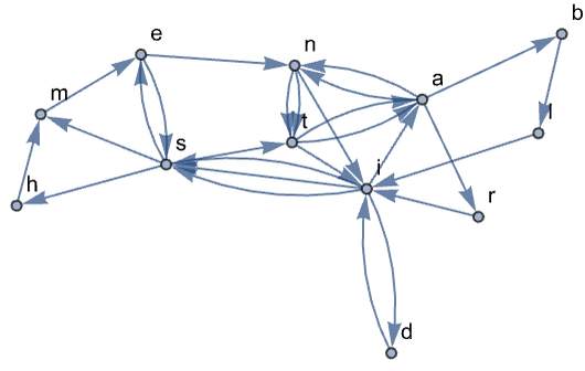
Here’s an example of how @@@ can help construct a graph from a list of pairs.
This generates a list of pairs of characters:
In[40]:=
Out[40]=
Turn this into a list of rules:
In[41]:=
Out[41]=
Form a transition graph showing how letters follow each other:
In[1437]:=
Out[1437]=
| FullForm[expr] | show full internal form | |
| TreeForm[expr] | show tree structure | |
| Head[expr] | extract the head of an expression | |
| _head | match any expression with a particular head | |
| f@@list | replace the head of list with f | |
| f@@@{list1,list2, ...} | replace heads of list1, list2, ... with f |


33.4Make a list of expression trees for the results of 4 successive applications of #^#& starting from x. »
33.7Generate a graph showing which word can follow which in the first 200 words of the Wikipedia article on computers. »
f@@expr is Apply[f, expr]. f@@@expr is MapApply[f, expr] or Apply[f, expr, {1}]. They’re usually just read as “double at” and “triple at”.
Are all expressions in the Wolfram Language trees?
At a structural level, yes. When there are variables with values assigned (see Section 38), though, they can behave more like directed graphs. And of course one can use Graph to represent any graph as an expression in the Wolfram Language.
- The basic concept of symbolic languages comes directly from work in mathematical logic stretching back to the 1930s and before, but other than in the Wolfram Language it’s been very rare for it to be implemented in practice.
- Wolfram Language expressions are a bit like XML expressions (and can be converted to and from them). But unlike XML expressions, Wolfram Language expressions can evaluate so that they automatically change their structure.
- Things like Select[f] that are set up to be applied to expressions are called operator forms, by analogy with operators in mathematics. Using Select[f][expr] instead of Select[expr, f] is often called currying, after a logician named Haskell Curry. OperatorApplied or CurryApplied let you “make operator forms” for anything. For example, OperatorApplied[f][x] applied to expr gives f[expr, x].
- Symbols like x can be used to represent algebraic variables or “unknowns”. This is central to doing many kinds of mathematics in the Wolfram Language.
- LeafCount gives the total number of atoms at the leaves of an expression tree. ByteCount gives the number of bytes needed to store the expression.
- ExpressionTree generates a Tree object, on which many operations can be done. ExpressionGraph gives the tree for an expression as a Graph.