New in Wolfram
Mathematica
8: Nonparametric, Derived, and Formula Distributions
◄
previous
|
next
►
Core Algorithms
Visualize a Marginal Distribution
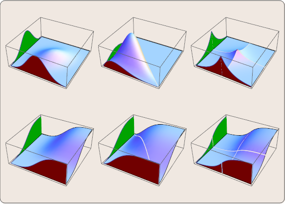
Visualize properties of the one-dimensional marginals of multivariate distributions, using
MarginalDistribution
.
In[1]:=
X
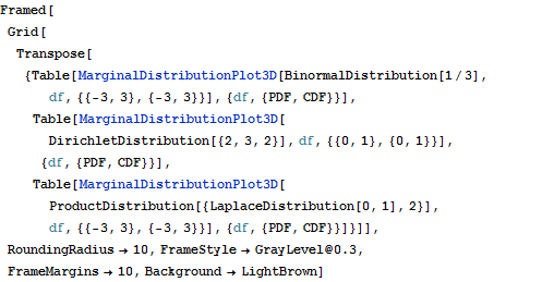
MarginalDistributionPlot3D[dist_, df_: PDF, {{xmin_, xmax_}, {ymin_, ymax_}}] := Module[{gxy, gx, gy}, gxy = Plot3D[ Evaluate@df[dist, {x, y}], {x, xmin, xmax}, {y, ymin, ymax}, Mesh -> None, PlotRange -> All]; gx = Plot[ Evaluate@df[MarginalDistribution[dist, 1], x], {x, xmin, xmax}, Filling -> Axis, FillingStyle -> Red]; gy = Plot[ Evaluate@df[MarginalDistribution[dist, 2], y], {y, ymin, ymax}, Filling -> Axis, FillingStyle -> Green]; Graphics3D[{First[gxy], First[gx] /. GraphicsComplex[pts_, rest__] :> GraphicsComplex[pts /. {x_, y_} -> {x, ymin, y}, rest], First[gy] /. GraphicsComplex[pts_, rest__] :> GraphicsComplex[pts /. {x_, y_} -> {xmin, x, y}, rest]}, BoxRatios -> {1, 1, 0.4}, ImageSize -> {178, 190}] ];
In[2]:=
X
Framed[Grid[ Transpose[{Table[ MarginalDistributionPlot3D[BinormalDistribution[1/3], df, {{-3, 3}, {-3, 3}}], {df, {PDF, CDF}}], Table[MarginalDistributionPlot3D[DirichletDistribution[{2, 3, 2}], df, {{0, 1}, {0, 1}}], {df, {PDF, CDF}}], Table[MarginalDistributionPlot3D[ ProductDistribution[{LaplaceDistribution[0, 1], 2}], df, {{-3, 3}, {-3, 3}}], {df, {PDF, CDF}}]}]], RoundingRadius -> 10, FrameStyle -> GrayLevel@0.3, FrameMargins -> 10, Background -> LightBrown]
Out[2]=