New in Wolfram
Mathematica
8: New and Improved Scientific and Information Visualization
◄
previous
|
next
►
Graphics & Visualization
Visualize Riemann Sums
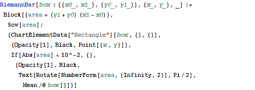
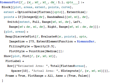
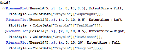
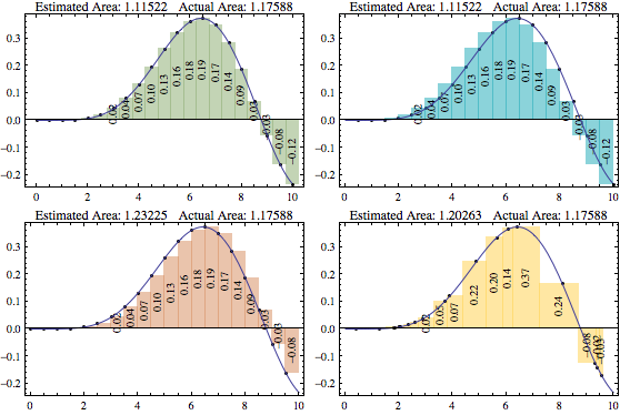
Riemann summation uses discrete rectangles to approximate the area under a curve or volume under a surface.
In[1]:=
X
RiemannBar[box : {{x0_, x1_}, {y0_, y1_}}, {x_, y_}, _] := Block[{area = (y1 + y0) (x1 - x0)}, Sow[area]; {ChartElementData["Rectangle"][box, {}, {}], {Opacity[1], Black, Point[{x, y}]}, If[Abs[area] < 10^-2, {}, {Opacity[1], Black, Text[Rotate[NumberForm[area, {Infinity, 2}], Pi/2], Mean /@ box]}]}]
In[2]:=
X
RiemannPlot[f_, {x_, x0_, x1_, dx_: 1.}, opts___] := Block[{plot, areas, extent, points, curve}, extent = OptionValue[Flatten[{opts}], ExtentSize]; points = If[IntegerQ[dx], RandomReal[{x0, x1}, dx], Switch[extent, Full, Range[x0, x1, dx], Left, Range[x0 + dx, x1, dx], Right, Range[x0, x1 - dx, dx]]]; {plot, areas} = Reap[DiscretePlot[f, Evaluate@{x, points}, opts, ImageSize -> 275, ExtentElementFunction -> RiemannBar, FillingStyle -> Opacity[0.5], PlotStyle -> PointSize[Medium]]]; Show[plot, Plot[f, {x, x0, x1}], PlotLabel -> Row[{"Estimated Area: ", Total[Flatten@areas], Spacer[10], "Actual Area: ", NIntegrate[f, {x, x0, x1}]}], Frame -> True, PlotRange -> All, Axes -> {True, False}] ]
In[3]:=
X
Grid[{{RiemannPlot[BesselJ[5, x], {x, 0, 10, 0.5}, ExtentSize -> Full, PlotStyle -> ColorData["Crayola"]["Asparagus"]], RiemannPlot[BesselJ[5, x], {x, 0, 10, 0.5}, ExtentSize -> Left, PlotStyle -> ColorData["Crayola"]["TealBlue"]]}, {RiemannPlot[ BesselJ[5, x], {x, 0, 10, 0.5}, ExtentSize -> Right, PlotStyle -> ColorData["Crayola"]["RawSienna"]], RiemannPlot[BesselJ[5, x], {x, 0, 10, 20}, ExtentSize -> Full, PlotStyle -> ColorData["Crayola"]["Sunglow"]]}}]
Out[3]=