Seed Random Number Generation and Visualization 

In[1]:=

X Needs["RLink`"] InstallR[]

Generate random normally distributed numbers with a fixed seed.

In[2]:=

X REvaluate["{ set.seed(123) rnorm(10,10) }"]

Out[2]=

Package this as a function.

In[3]:=

X rnormFixedSeed = RFunction["function(n, m = 0, sdev = 1, seed = 1){ set.seed(seed) rnorm(n,mean = m, sd= sdev) }"];

Test the function.

In[4]:=

X rnormFixedSeed[10]

Out[4]=

Since the seed is fixed, the same seed value always returns the same pseudo-random sequence.

In[5]:=

X rnormFixedSeed[10]

Out[5]=

Generate a set of random numbers.

In[6]:=

X (randR = rnormFixedSeed[10000]) // Short // AbsoluteTiming

Out[6]=

Test them for normality with Mathematica's QuantilePlot.

In[7]:=

X QuantilePlot[randR]

Out[7]=

And with EstimatedDistribution.

In[8]:=

X Clear[mu, sigma]; dist = EstimatedDistribution[randR, NormalDistribution[mu, sigma]]

Out[8]=

Visualize the result.

In[9]:=

X Show[Histogram[randR, Automatic, "ProbabilityDensity"], Plot[PDF[dist, x], {x, -5, 5}, PlotStyle -> Thick]]

Out[9]=

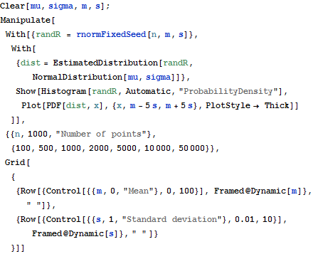
Use the dynamic interactivity of Mathematica for data analysis. The random numbers are generated in R but analyzed and visualized in Mathematica.

In[10]:=

X Clear[mu, sigma, m, s]; Manipulate[ With[{randR = rnormFixedSeed[n, m, s]}, With[{dist = EstimatedDistribution[randR, NormalDistribution[mu, sigma]]}, Show[Histogram[randR, Automatic, "ProbabilityDensity"], Plot[PDF[dist, x], {x, m - 5 s, m + 5 s}, PlotStyle -> Thick]] ]], {{n, 1000, "Number of points"}, {100, 500, 1000, 2000, 5000, 10000, 50000}}, Grid[ { {Row[{Control[{{m, 0, "Mean"}, 0, 100}], Framed@Dynamic[m]}, " "]}, {Row[{Control[{{s, 1, "Standard deviation"}, 0.01, 10}], Framed@Dynamic[s]}, " " ]} }]]

Out[10]=