Model Differences in Log Returns of Stock Prices 

Consider differences in log returns for Google stocks.

In[1]:=

X goog = Differences[ Log[FinancialData["GOOG", {{2008, 3, 10}, {2010, 3, 15}, "Day"}, "Value"]]];

Fit a TsallisQGaussianDistribution to the data and compare against the fit with a NormalDistribution.

In[2]:=

X edist1 = EstimatedDistribution[goog, TsallisQGaussianDistribution[\[Mu], \[Beta], q]]

Out[2]=

In[3]:=

X edist2 = EstimatedDistribution[goog, NormalDistribution[\[Mu], \[Sigma]]]

Out[3]=

In[4]:=

X DistributionFitTest[goog, #] & /@ {edist1, edist2}

Out[4]=

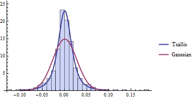
Compare a histogram of the data to the PDF of the fitted distributions.

In[5]:=

X h = Histogram[goog, 30, "PDF"]; pdfs = Plot[{PDF[edist1, x], PDF[edist2, x]}, {x, -0.1, .1}, PlotStyle -> Thick, PlotLegends -> {"Tsallis", "Gaussian"}]; Show[{h, pdfs}, ImageSize -> 300]

Out[5]=

Inspect the heavy-tail behavior.

In[6]:=

X {QuantilePlot[goog, edist1], QuantilePlot[goog, edist2]}

Out[6]=

Find the probability of the log-return to exceed 0.10.

In[7]:=

X Probability[x > 0.1, x \[Distributed] edist1]

Out[7]=

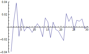
Simulate the log difference in price for 30 consecutive days.

In[8]:=

X ListLinePlot[RandomVariate[edist1, 30], ImageSize -> 300]

Out[8]=