Accuracy of Approximation Schemes 

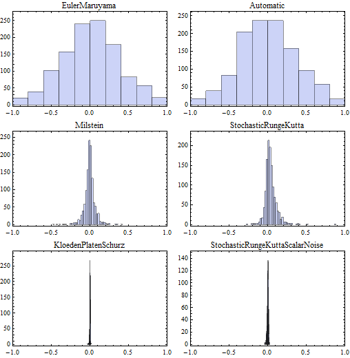
Sampling from ItoProcess and StratonovichProcess generically uses strong approximation schemes of different orders of convergence.

Consider a vector-valued Ito process with components and and convert it to a standard Ito process.

In[1]:=

X pr = ItoProcess[ ItoProcess[{0, 1, {w[t], w[t]^4 - 6 w[t]^2 t + 3 t^2}}, w, t]]

Out[1]=

Sample from the standard Ito process using different approximation schemes, and measure the residuals with the exact function of the Wiener process.

In[2]:=

X residuals[mthd_] := Block[{td}, td = RandomFunction[pr, {0., 1, .01}, 1250, Method -> mthd]; Histogram[ Function[{x, y}, y - (x^4 - 6 x^2 + 3)] @@@ Part[td["States"], All, -1], ImageSize -> 250, PlotRange -> {{-1, 1}, Automatic}, PlotRangeClipping -> True, PlotLabel -> mthd, Frame -> True, Axes -> False]]

In[3]:=

X {{residuals["EulerMaruyama"], residuals[Automatic]}, {residuals["Milstein"], residuals["StochasticRungeKutta"]}, {residuals["KloedenPlatenSchurz"], residuals["StochasticRungeKuttaScalarNoise"]}} // Grid

Out[3]=