Simulate Time Series Data 

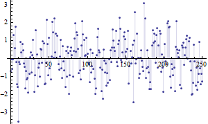
Any time series process in Mathematica can be used to simulate random time series data. Use ARProcess, MAProcess, or ARMAProcess to simulate a weakly stationary time series.

In[1]:=

X RandomFunction[ARMAProcess[{.1, .2}, {.3, -.2}, 1], {0, 250}]; ListPlot[%, Filling -> Axis]

Out[1]=

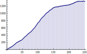
Use ARIMAProcess to simulate a time series with a trend.

In[2]:=

X RandomFunction[ARIMAProcess[{-.7}, 2, {.2}, 1], {0, 250}]; ListPlot[%, Filling -> Axis]

Out[2]=

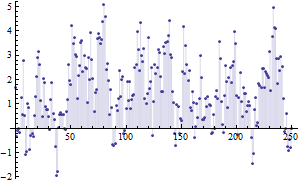
Use SARMAProcess or SARIMAProcess to simulate seasonal time series.

In[3]:=

X RandomFunction[ SARIMAProcess[{.4}, 1, {-1.3}, {12, {.7, .3}, 2, {.7, -.3}}, 1], {0, 250}]; ListPlot[%, Filling -> Axis]

Out[3]=

Use FARIMAProcess to simulate a long memory time series.

In[4]:=

X RandomFunction[FARIMAProcess[{.1}, .45, {.2}, 1], {0, 250}]; ListPlot[%, Filling -> Axis]

Out[4]=