스미스 분해를 사용한 격자 분석

벡터 과 의 배수인 정수에 의해 생성된 격자 을 검토해 봅니다.

In[1]:=

b1 = {3, -3}; b2 = {2, 1};

In[2]:=

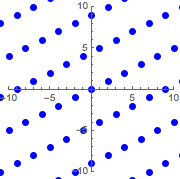
ptsb = Flatten[Table[j b1 + k b2, {j, -12, 12}, {k, -12, 12}], 1];

In[3]:=

graphicsb = Graphics[{Blue, PointSize[Large], Point@ptsb}, PlotRange -> 10, Axes -> True]

Out[3]=

을 행이 과 의 행렬로 합니다.

In[4]:=

m = {b1, b2};

스미스 분해는 항등식 을 만족하는 3개의 행렬을 줍니다.

In[5]:=

{u, r, v} = SmithDecomposition[m];

In[6]:=

u.m.v == r

Out[6]=

행렬 와 는 정수의 요소와 행렬식 1을 가집니다.

In[7]:=

{u // MatrixForm, v // MatrixForm, Det[u], Det[v]}

Out[7]=

행렬 은 정수이며 대각 행렬입니다. 그 항목에서 의 군의 구조는 또는 간단히 이며, 은 자명군입니다.

In[8]:=

r // MatrixForm

Out[8]//MatrixForm=

항등식 을 에 곱하면, 이 됩니다. 는 정수이며, 행렬식은 1이므로, 는 과 같은 격자를 생성하지만, 훨씬 간단합니다.

In[9]:=

g = r.Inverse[v]; g // MatrixForm

Out[9]//MatrixForm=

행에 의해 생성된 격자를 시각화합니다.

In[10]:=

ptsg = Flatten[ Table[j First[g] + k Last[g], {j, -12, 12}, {k, -12, 12}], 1];

In[11]:=

graphicsg = Graphics[{Red, PointSize[Medium], Point@ptsg}, PlotRange -> 10, Axes -> True]

Out[11]=

새로운 격자를 오리지널 격자에 겹쳐 놓으면 모두 동일한지 확인할 수 있습니다.

In[12]:=

Show[{graphicsb, graphicsg}]

Out[12]=