Model Constrained Systems as DAEs 

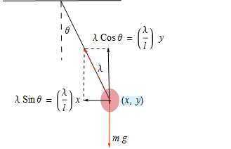
Model the motion of a single pendulum.

X \!\(\* GraphicsBox[{ LineBox[{{0.31643990929705235`, 0.9233333333333335}, { 1.0142176870748305`, 0.9255555555555556}}], LineBox[{{0.6589503579209464, 0.9232083333333333}, { 0.9520953937130411, 0.45005429292929255`}}], {EdgeForm[{GrayLevel[0.], Opacity[1.], AbsoluteThickness[1]}], EdgeForm[None], FaceForm[{RGBColor[0.750454, 0.0792859, 0.15021], Opacity[0.41000000000000003`]}], DiskBox[{0.9500000000000002, 0.45444444444444443`}, 0.05555555555555558]}, {StrokeForm[Hue[0.027777777777777776`, 0.972972972972973, 1.]], EdgeForm[{RGBColor[0., 0., 0.], Opacity[1.], AbsoluteThickness[ 1]}], EdgeForm[None], FaceForm[{RGBColor[ 0.750454, 0.0792859, 0.15021], Opacity[0.41000000000000003`]}], ArrowBox[{{0.946572407883462, 0.46028277634961445`}, { 0.9443501856612398, 0.22917166523850319`}}]}, {EdgeForm[{GrayLevel[0.], Opacity[1.], AbsoluteThickness[1]}], EdgeForm[None], FaceForm[{RGBColor[0.750454, 0.0792859, 0.15021], Opacity[0.41000000000000003`]}], ArrowBox[{{0.9454136585834917, 0.43798390155505434`}, { 0.9380052507458762, 0.7050877266916664}}]}, {EdgeForm[{GrayLevel[0.], Opacity[1.], AbsoluteThickness[1]}], EdgeForm[None], FaceForm[{RGBColor[0.750454, 0.0792859, 0.15021], Opacity[0.41000000000000003`]}], ArrowBox[{{0.9499104847594564, 0.45444444444444265`}, { 0.789513659362631, 0.45444444444444265`}}]}, {Dashing[{Medium, Medium}], StrokeForm[Hue[ 0.038888888888888896`, 1., 0.8968210694173823]], EdgeForm[{ RGBColor[0., 0., 0.], Opacity[1.], AbsoluteThickness[1]}], EdgeForm[None], FaceForm[{RGBColor[0.750454, 0.0792859, 0.15021], Opacity[0.41000000000000003`]}], ArrowBox[{{0.9481916220444971, 0.4523053737130471}, { 0.7970110400803492, 0.700978340384216}}]}, StyleBox[InsetBox[ StyleBox[\[Lambda], Background->GrayLevel[ 1.]], {0.8799457297914878, 0.5849900028563257}, { Left, Baseline}, Alignment->{Left, Top}], FontSize->14], StyleBox[InsetBox[ RowBox[{ StyleBox[ RowBox[{"\[Lambda]", " ", "Cos", " ", "\[Theta]"}], Background->GrayLevel[1.]], StyleBox[" ", Background->GrayLevel[1.]], StyleBox["=", Background->GrayLevel[1.]], StyleBox[" ", Background->GrayLevel[1.]], RowBox[{ RowBox[{ StyleBox["(", Background->GrayLevel[1.]], FractionBox["\[Lambda]", "l"], ")"}], " ", "y", StyleBox[, Background->GrayLevel[ 1.]]}]}], {0.8506016079714928, 0.7313656051432611}, { Left, Baseline}, {0.6086703096539166, 0.13846994535519133`}, {{ 1., 0.}, {0., 1.}}, Alignment->{Left, Top}], FontSize->14], StyleBox[InsetBox[ StyleBox[ TagBox[ RowBox[{ RowBox[{"\[Lambda]", " ", "Sin", " ", "\[Theta]"}], " ", "=", " ", RowBox[{ RowBox[{"(", FractionBox["\[Lambda]", "l"], ")"}], " ", "x"}]}], "RawBoxes"], Background->GrayLevel[ 1.]], {0.3892059411596686, 0.43888888888888733`}, { Left, Baseline}, {0.5270494144530135, 0.13668666095401316`}, {{ 1., 0.}, {0., 1.}}, Alignment->{Left, Top}], FontSize->14], InsetBox[ StyleBox[ TagBox[ RowBox[{"m", " ", "g"}], "RawBoxes"], FontSize->14, Background->GrayLevel[ 1.]], {0.9675488735081297, 0.25563364433949665`}, { Left, Baseline}, Alignment->{Left, Top}], InsetBox[ StyleBox[ TagBox["\[Theta]", "RawBoxes"], FontSize->14, Background->GrayLevel[ 1.]], {0.6899340235342597, 0.7652122812685833}, { Left, Baseline}, Alignment->{Left, Top}], {Dashing[{Small, Small}], LineBox[{{0.8036507841613358, 0.6970865467009446}, { 0.9407544688228608, 0.6970865467009437}}]}, {Dashing[{Small, Small}], LineBox[{{0.7969151670951157, 0.6970865467009455}, { 0.7934875749785772, 0.4537275064267372}}]}, {Dashing[{Medium, Medium}], LineBox[{{0.6598114824335904, 0.9198800342759241}, { 0.6632390745501283, 0.6456726649528728}}]}, InsetBox["", {1.0368466152527849`, 0.4365895458440474}, { Left, Baseline}, Alignment->{Left, Top}], InsetBox[ StyleBox[ TagBox[ RowBox[{"(", RowBox[{"x", ",", "y"}], ")"}], "RawBoxes"], FontSize->14, Background->RGBColor[ 0.8500038147554742, 0.9499961852445258, 1.]], {1.0197086546700942`, 0.4365895458440474}, { Left, Baseline}, Alignment->{Left, Top}]}, AspectRatio->Full, ImagePadding->{{0., 147.937294}, {1., 0.}}, ImageSize->{328.890625, 212.}, PlotRange->{{0.3014314362563079, 1.0518550882935294`}, { 0.22555597697878604`, 0.925555134132325}}, PlotRangePadding->Automatic]\)

Derive the governing equations using Newton's second law of motion, and .

In[1]:=

X deqns = {m x''[t] == (\[Lambda][t]/l) x[t], m y''[t] == (\[Lambda][t]/l) y[t] - m g};

Express the fixed length of the pendulum rod as an algebraic constraint.

In[2]:=

X aeqns = {x[t]^2 + y[t]^2 == l^2};

The pendulum is released from the horizontal position with a vertical velocity of 1.

In[3]:=

X ics = {x[0] == 1, y[0] == 0, x'[0] == 0, y'[0] == 1};

Specify the physical parameters for the pendulum system.

In[4]:=

X params = {g -> 9.81, m -> 1, l -> 1};

Solve the high-index DAE and visualize the system.

In[5]:=

X pendulumSol = First[NDSolve[{deqns, aeqns, ics} /. params, {x, y, \[Lambda]}, {t, 0, 15}, Method -> {"IndexReduction" -> Automatic}]];

In[6]:=

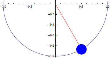
X Show[{ParametricPlot[ Evaluate[{x[t], y[t]} /. pendulumSol], {t, 0, 15}, PlotStyle -> {DotDashed}], Graphics[{{Red, Line[{{0, 0}, {0.5, -Sqrt[3]/2}}]}, {Blue, Disk[{0.5, -Sqrt[3]/2}, 0.1]} }]}, ImageSize -> Medium]

Out[6]=