Analyze the Performance of a Queueing Network 

Define an open queueing network.

In[1]:=

X \[Gamma] = {3, 6}; \[Mu] = {7, 17}; r = {{1/6, 1/9}, {1/4, 1/8}}; c = {1, 1};

In[2]:=

X \[ScriptCapitalN] = QueueingNetworkProcess[\[Gamma], r, \[Mu], c];

Simulate the network.

In[3]:=

X data = RandomFunction[\[ScriptCapitalN], {0, 10}];

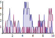
Plot the simulated values at the nodes in the network.

In[4]:=

X ListLinePlot[data, Filling -> Axis]

Out[4]=

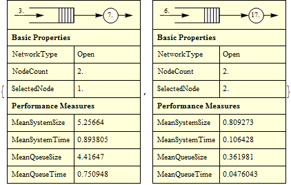
Performance measures at the nodes in the network.

In[5]:=

X Table[QueueProperties[{\[ScriptCapitalN], i}], {i, 2}] // N

Out[5]=

Stationary distribution for the network.

In[6]:=

X \[ScriptCapitalD] = StationaryDistribution[\[ScriptCapitalN]];

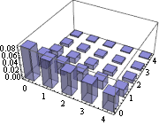
Probability density function for the steady state of the network.

In[7]:=

X PDF[\[ScriptCapitalD], {m, n}]

Out[7]=

In[8]:=

X DiscretePlot3D[ PDF[\[ScriptCapitalD], {m, n}] // Evaluate, {m, 0, 4}, {n, 0, 4}, ExtentSize -> 0.5, PlotRange -> All]

Out[8]=

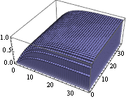
Cumulative distribution function for the steady state of the network.

In[9]:=

X CDF[\[ScriptCapitalD], {m, n}]

Out[9]=

In[10]:=

X DiscretePlot3D[ CDF[\[ScriptCapitalD], {m, n}] // Evaluate, {m, 0, 35}, {n, 0, 35}, ExtentSize -> Right, PlotRange -> {0, 1.05}]

Out[10]=