Simulate Different Types of Queues 

Simulate an M/M/1 queue in which customers arrive at the rate of three per hour and are served at the rate of five per hour.

In[1]:=

X data = RandomFunction[QueueingProcess[3, 5], {0, 20}]

Out[1]=

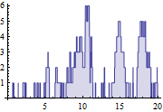
Since the arrival rate is less than the service rate, the system reaches a steady state.

In[2]:=

X ListLinePlot[data, InterpolationOrder -> 0, Filling -> Axis]

Out[2]=

If the arrival rate is greater than the service rate, then the system does not reach a steady state.

In[3]:=

X data = RandomFunction[QueueingProcess[5, 3], {0, 150}];

In[4]:=

X ListLinePlot[data, Filling -> Axis]

Out[4]=

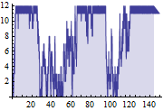
Simulate a queueing system that can hold only 12 customers.

In[5]:=

X data = RandomFunction[QueueingProcess[6, 6.1, 1, 12], {0, 150}];

In[6]:=

X ListLinePlot[data, Filling -> Axis]

Out[6]=

Simulate a queue with 20 customers in the initial state.

In[7]:=

X data = RandomFunction[ QueueingProcess[2, 3, 1, \[Infinity], 20], {0, 80}];

In[8]:=

X ListLinePlot[data, InterpolationOrder -> 0, Filling -> Axis, PlotRange -> All]

Out[8]=