Sensitivity of the Duffing Equation 

Explore the sensitivity of the Duffing equation to initial conditions.

To simplify the computations that follow, use ParametricNDSolveValue with only the initial conditions as parameters and other values fixed.

In[1]:=

X xp = ParametricNDSolveValue[{x''[ t] + \[Delta] x'[t] + \[Alpha] x[ t] + \[Beta] x[t]^3 == \[Gamma] Cos[\[Omega] t], x[0] == a, x'[0] == b} /. {\[Delta] -> 0.15, \[Alpha] -> -1, \[Beta] -> 1, \[Gamma] -> 0.3, \[Omega] -> 1}, x, {t, 0, 100}, {a, b}]

Out[1]=

The derivatives of the ParametricFunction with respect to a and b are the sensitivities with respect to the initial values for x and its derivative x, respectively.

In[2]:=

X {xpa = Head[D[xp[a, b], a]], xpb = Head[D[xp[a, b], b]]}

Out[2]=

Show a plot of the solution starting at {0, 0} and log plots of the sensitivities.

In[3]:=

X GraphicsRow[{Plot[xp[0, 0][t], {t, 0, 100}], LogPlot[Abs[xpa[0, 0][t]], {t, 0, 100}], LogPlot[Abs[xpb[0, 0][t]], {t, 0, 100}]}]

Out[3]=

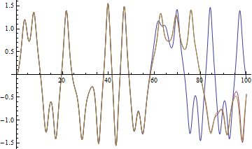
The enormous sensitivities indicate that even a small change in either of these parameters will lead to a large deviation in the solution. Shown below are the solutions with a small perturbation from the origin in either direction.

In[4]:=

X \[Epsilon] = 10^-6; Plot[{xp[0, 0][t], xp[\[Epsilon], 0][t], xp[0, \[Epsilon]][t]}, {t, 0, 100}, ImageSize -> Medium]

Out[4]=

Another way to visualize the sensitivity is to locally break it down into components parallel and perpendicular to the direction of the trajectory in the phase plane.

Define a function that gives a vector perpendicular to the trajectory as a function of time.

In[5]:=

X perp[a_, b_][t_?NumberQ] := Module[{f = xp[a, b], dt, do}, dt = Normalize[{f'[t], f''[t]}]; do = Reverse[dt]*{1, -1} ];

Now define functions that give the magnitude of the components of the sensitivity with respect to the initial value of x in the parallel and perpendicular directions.

In[6]:=

X spar[a_, b_][t_?NumberQ] := Module[{s = xpa[a, b], f = xp[a, b]}, Abs[Normalize[{f'[t], f''[t]}].{s[t], s'[t]}]]

In[7]:=

X sperp[a_, b_][t_?NumberQ] := Module[{s = xpa[a, b]}, Abs[perp[a, b][t].{s[t], s'[t]}]]

For this equation, the two components grow at comparable rates.

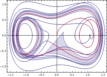
The component breakdown allows a nice visualization in the phase plane. Changing the scaling of the sensitivity makes it possible to see it for different time intervals.

In[8]:=

X scale = 10^-8; Show[ ParametricPlot[{xp[0, 0][t], xp[0, 0]'[t]} + s sperp[0, 0][t] perp[0, 0][t], {t, 0, 100}, {s, -scale, scale}, Mesh -> None, PlotPoints -> {1000, 2}], ParametricPlot[{xp[0, 0][t], xp[0, 0]'[t]}, {t, 0, 25}, PlotStyle -> Red], ImageSize -> Medium]

Out[8]=