Compute Parametric Sensitivities 

In[2]:=

X Show[Plot[Evaluate@Table[pfun[a][t], {a, -.6, .6, .1}], {t, 0, 5}, PlotStyle -> Lighter[Gray, 0.3], PlotRange -> All], Plot[pfun[0][t], {t, 0, 5}, PlotStyle -> {Lighter[Black, .4], Thick}], ImageSize -> Medium]

In[3]:=

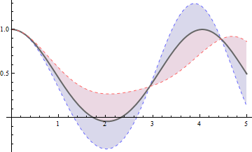
X Plot[Evaluate[pfun[0][t] + {-.5, 0, .5} pfun'[0][t]], {t, 0, 5}, PlotStyle -> {{Dashed, Lighter[Blue, .4]}, {Thick, Lighter[Black, .4]}, {Dashed, Lighter[Red, .4]}}, Filling -> {1 -> {2}, 2 -> {3}}, ImageSize -> Medium]

Perturbing a parameter in the differential equation gives a family of solutions.

In[1]:=

X pfun = ParametricNDSolveValue[{y''[t] + y[t] == a Sin[2 t ] + Cos[2 y[t]], y[0] == 1, y'[0] == 0}, y, {t, 0, 10}, {a}];

Out[2]=

Sensitivity solutions clearly show the effect of small changes in the parameter.

Out[3]=