« View all new features in
Mathematica
9
◄
previous
|
next
►
New in
Mathematica
9
›
Parametric Differential Equations
Newton's Law of Cooling
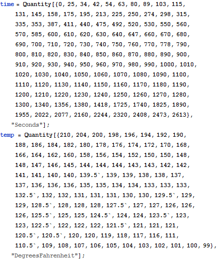
Fit data sampled from a container of cooling liquid to the model from Newton's law of cooling.
In[1]:=
X
time = Quantity[{0, 25, 34, 42, 54, 63, 80, 89, 103, 115, 131, 145, 158, 175, 195, 213, 225, 250, 274, 298, 315, 335, 353, 387, 411, 440, 475, 492, 520, 530, 550, 560, 570, 585, 600, 610, 620, 630, 640, 647, 660, 670, 680, 690, 700, 710, 720, 730, 740, 750, 760, 770, 778, 790, 800, 810, 820, 830, 840, 850, 860, 870, 880, 890, 900, 910, 920, 930, 940, 950, 960, 970, 980, 990, 1000, 1010, 1020, 1030, 1040, 1050, 1060, 1070, 1080, 1090, 1100, 1110, 1120, 1130, 1140, 1150, 1160, 1170, 1180, 1190, 1200, 1210, 1220, 1230, 1240, 1250, 1260, 1270, 1280, 1300, 1340, 1356, 1380, 1418, 1725, 1740, 1825, 1890, 1955, 2022, 2077, 2160, 2244, 2320, 2408, 2473, 2613}, "Seconds"]; temp = Quantity[{210, 204, 200, 198, 196, 194, 192, 190, 188, 186, 184, 182, 180, 178, 176, 174, 172, 170, 168, 166, 164, 162, 160, 158, 156, 154, 152, 150, 150, 148, 148, 147, 146, 145, 144, 144, 144, 143, 143, 142, 142, 141, 141, 140, 140, 139.5, 139, 139, 138, 138, 137, 137, 136, 136, 136, 135, 135, 134, 134, 133, 133, 133, 132.5, 132, 132, 131, 131, 131, 130, 130, 129.5, 129, 129, 128.5, 128, 128, 128, 127.5, 127, 127, 126, 126, 126, 125.5, 125, 125, 124.5, 124, 124, 123.5, 123, 123, 122.5, 122, 122, 122, 121.5, 121, 121, 121, 120.5, 120.5, 120, 120, 119, 118, 117, 116, 111, 110.5, 109, 108, 107, 106, 105, 104, 103, 102, 101, 100, 99}, "DegreesFahrenheit"];
Convert data to kelvins and find initial and final (ambient) temperatures.
In[2]:=
X
tempK = UnitConvert[temp, "Kelvins"]; Subscript[tempK, 0] = QuantityMagnitude[First[tempK]]; Subscript[tempK, \[Infinity]] = QuantityMagnitude[ UnitConvert[Quantity[79, "DegreesFahrenheit"], "Kelvins"]]; tend = QuantityMagnitude[Last[time]];
Find solutions to Newton's law of cooling depending on parameters
k1
and
k2
.
In[3]:=
X
BoltzmannConstant = Quantity[1.3806504`*^-23 , "Joules"/"Kelvins"]; c = QuantityMagnitude[(2260 18)/(6.02 10^23 BoltzmannConstant)];
In[4]:=
X
pfun = ParametricNDSolveValue[{(Derivative[1][T][ t] == -k1 (T[t] - Subscript[tempK, \[Infinity]]) - k2 (E^(-c/T[t]) - E^(-c/Subscript[tempK, \[Infinity]]))), T[0] == Subscript[tempK, 0]}, T, {t, 0, tend}, {k1, k2}];
Fit the parameters in the differential equation to the given data.
In[5]:=
X
fitdata = N@QuantityMagnitude[Transpose[{time, tempK}]];
In[6]:=
X
fit = FindFit[fitdata, pfun[k1, k2][t], {{k1, 0.0001}, {k2, 10000}}, t]
Out[6]=
Show the solution with the data.
In[7]:=
X
Show[ ListPlot[fitdata], Plot[Evaluate[pfun[k1, k2][t] /. fit], {t, 0, tend}, PlotStyle -> Red], ImageSize -> Medium]
Out[7]=