Simulation of Processes Driven by a Vector Noise Process 

Define a scalar process driven by two independent Wiener noise processes.

In[1]:=

X pr = ItoProcess[\[DifferentialD]x[ t] == -x[t]/(\[Sqrt](1 + x[t]^2)) \[DifferentialD]t + Sin[x[t]] \[DifferentialD]w1[t] + Cos[x[t]] \[DifferentialD]w2[t], x[t], {x, 0}, t, {w1 \[Distributed] WienerProcess[], w2 \[Distributed] WienerProcess[]}]

Out[1]=

Simulate the process using the Milstein scheme.

In[2]:=

X paths = RandomFunction[pr, {0, 4 Pi, 0.01}, 250, Method -> "Milstein"]

Out[2]=

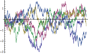
Visualize five sample trajectories.

In[3]:=

X ListLinePlot[paths["Part", 1 ;; 5], ImageSize -> 300]

Out[3]=

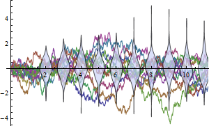
Show the sample trajectories with slice distributions at various times.

In[4]:=

X plot1 = ListLinePlot[paths["Part", 1 ;; 12]]; plot2 = DistributionChart[ Transpose@(paths["SliceData", Range[0, 4 Pi, 1.1]]), ChartStyle -> Opacity[0.7]]; Show[plot1, plot2, PlotRange -> {{0, 11}, Automatic}, ImageSize -> 300]

Out[4]=