Ito and Stratonovich Solutions of the Linear Growth Model 

Define ItoProcess and StatonovichProcess for the SDE .

In[1]:=

X ipr = ItoProcess[\[DifferentialD]x[t] == x[t] (r \[DifferentialD]t + \[Sigma] \[DifferentialD]w[t]), x[t], {x, x0}, t, w \[Distributed] WienerProcess[]]

Out[1]=

In[2]:=

X spr = StratonovichProcess[\[DifferentialD]x[t] == x[t] (r \[DifferentialD]t + \[Sigma] \[DifferentialD]w[t]), x[t], {x, x0}, t, w \[Distributed] WienerProcess[]]

Out[2]=

Find the mean and variance functions for the Ito process.

In[3]:=

X {Mean[ipr[t]], Variance[ipr[t]]} // Simplify

Out[3]=

The mean and variance functions for the Stratonovich process are different.

In[4]:=

X {Mean[spr[t]], Variance[spr[t]]} // Simplify

Out[4]=

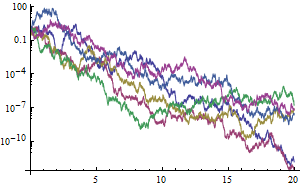
When , the Ito solution converges to zero almost surely.

In[5]:=

X Assuming[0 < r < \[Sigma]^2/2 && \[Sigma] > 0 && x0 > 0, Limit[Probability[ 0 < \[FormalX][t] <= 1/t, \[FormalX] \[Distributed] ipr], t -> \[Infinity]]]

Out[5]=

Confirm the convergence to zero using simulations.

In[6]:=

X ListLogPlot[ RandomFunction[ ipr /. {r -> 1, \[Sigma] -> 2, x0 -> 1}, {0, 20., 0.002}, 6, Method -> "KPS"], PlotRange -> All, Joined -> True, ImageSize -> 300]

Out[6]=

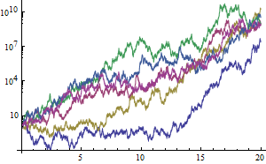
When , the Stratonovich solution, however, diverges almost surely.

In[7]:=

X Assuming[0 < r < \[Sigma]^2/2 && \[Sigma] > 0 && x0 > 0, Limit[Probability[\[FormalX][t] > t, \[FormalX] \[Distributed] spr], t -> \[Infinity]]]

Out[7]=

Confirm the divergence using simulations.

In[8]:=

X ListLogPlot[ RandomFunction[ spr /. {r -> 1, \[Sigma] -> 2, x0 -> 1}, {0, 20., 0.002}, 6, Method -> "KPS"], PlotRange -> All, Joined -> True, ImageSize -> 300]

Out[8]=