Stochastic Logistic Growth Model 

Define the SDE describing the stochastic logistic growth model.

In[1]:=

X slgm[r_, xmax_, x0_, \[Sigma]_] := ItoProcess[\[DifferentialD]x[t] == x[t] (1 - x[t]/ xmax) (r \[DifferentialD]t + \[Sigma] \[DifferentialD]w[t]), x[t], {x, x0}, t, w \[Distributed] WienerProcess[]]

The deterministic solution corresponding to is well known.

In[2]:=

X detsol[r_, xmax_, x0_] := Function[t, ((E^(r t)) x0 )/((E^(r t) - 1) x0/xmax + 1)]

Simulate the SDE using the method of Kloeden-Platen-Schurz of strong order .

In[3]:=

X stochsol[r_, xmax_, x0_, \[Sigma]_] := RandomFunction[slgm[r, xmax, x0, \[Sigma]], {0, 6, 0.005}, 10, Method -> "KloedenPlatenSchurz"]

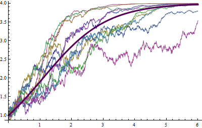
Visualize stochastic and deterministic solutions.

In[4]:=

X With[{r = 1, xmax = 4, x0 = 1, \[Sigma] = 1/2}, Show[ListLinePlot[stochsol[r, xmax, x0, \[Sigma]]], Plot[detsol[r, xmax, x0][t], {t, 0, 6}, PlotStyle -> Directive[Darker@Purple, Thickness[.008]]], ImageSize -> 400]]

Out[4]=