Word Frequency over Time
Version 11 introduces WordFrequencyData to collect information on word frequencies from published texts, in multiple languages. Use this new function to track trends in the usage of words over time.
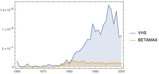
Compare the use of the names of two video formats between the years 1960 and 2000.
In[1]:=
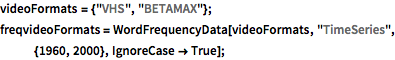
videoFormats = {"VHS", "BETAMAX"};
freqvideoFormats =
  WordFrequencyData[videoFormats, "TimeSeries", {1960, 2000},
   IgnoreCase -> True];
In[2]:=
DateListPlot[freqvideoFormats, Filling -> Axis]Out[2]=
Compare the use of the names of these transportation methods over two centuries.
In[3]:=
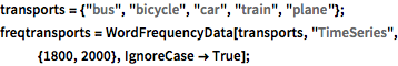
transports = {"bus", "bicycle", "car", "train", "plane"};
freqtransports =
  WordFrequencyData[transports, "TimeSeries", {1800, 2000},
   IgnoreCase -> True];
In[4]:=
DateListPlot[freqtransports, Filling -> Axis]Out[4]=
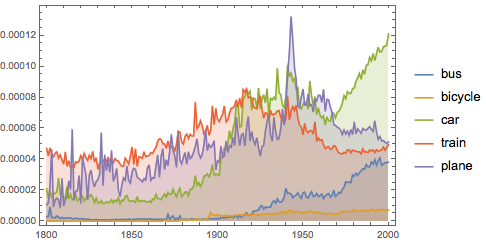
Discover when the pen became mightier than the sword.
In[5]:=
DateListPlot[
 WordFrequencyData[{"sword", "pen"}, "TimeSeries", {1700, 2000},
  IgnoreCase -> True], Filling -> Axis]
Out[5]=
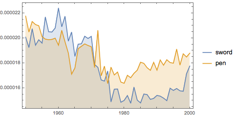
Reduce the time window to find out when the sword began to make a comeback.
In[6]:=
DateListPlot[
 WordFrequencyData[{"sword", "pen"}, "TimeSeries", {1950, 2000},
  IgnoreCase -> True], Filling -> Axis]
Out[6]=