Visualize Eigenfunctions

Define a 3D Laplacian operator.

In[1]:=

\[ScriptCapitalL] = -Laplacian[u[x, y, z], {x, y, z}];

Specify homogeneous Dirichlet boundary conditions.

In[2]:=

\[ScriptCapitalB] = DirichletCondition[u[x, y, z] == 0, True];

Find the smallest eigenvalues and eigenfunctions in a ball.

In[3]:=

\[CapitalOmega] = Ball[{0, 0, 0}, 2]; {vals, funs} = DEigensystem[{\[ScriptCapitalL], \[ScriptCapitalB]}, u[x, y, z], {x, y, z} \[Element] \[CapitalOmega], 2];

In[4]:=

funs

Out[4]=

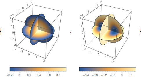
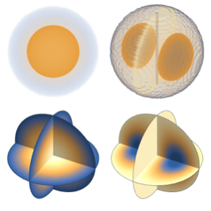
Plot each eigenfunction using a 3D density plot.

In[5]:=

Table[DensityPlot3D[ Evaluate[N[f]], {x, y, z} \[Element] \[CapitalOmega], PlotTheme -> "NoAxes", PlotLegends -> Placed[Automatic, Below]], {f, funs}]

Out[5]=

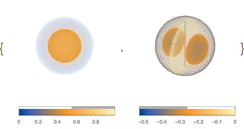
Use coordinate planes to plot the density.

In[6]:=

Table[SliceDensityPlot3D[ Evaluate[N[f]], {x, y, z} \[Element] \[CapitalOmega], PlotLegends -> Placed[Automatic, Below]], {f, funs}]

Out[6]=