Segmentation of a Knee Bone in 3D
To quantify and measure the properties of a component in a volume, segmentation is a necessary first step. To segment the bone tissue in an MRT volume, a clustering algorithm is used to achieve a rough segmentation and apply a grow-cut algorithm to obtain the final result.
| Out[1]= |  |
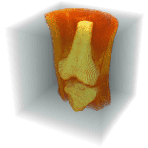
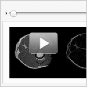
The volume is preprocessed using MedianFilter to regularize noise. An initial segmentation is performed by clustering voxel intensities using ClusteringComponents. This partitions the data into three regions: empty space, muscle tissue, and the rest, which includes bone, fat, and skin.
| Out[2]= |  |
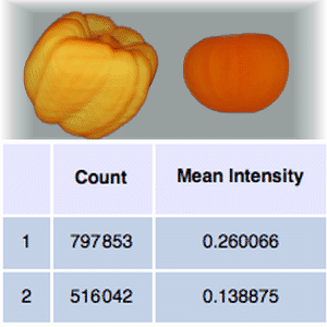
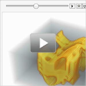
Extract the segment with highest mean intensity, which depicts bone, fat, and skin tissue.
| Out[3]= |  |
| Out[4]= | 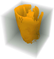 |
GrowCutComponents can provide a nice final segmentation. In order to create two markers for bone and no-bone areas, one can use morphological operations.
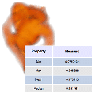
The bone marker can be computed by eroding the segment using a radius 4, which deletes all thin skin and fat layers and also erodes some of the bone.
| Out[5]= |  |
For the no-bone marker, dilate the bone core more than what was eroded and extract the surface around the dilated volume.
| Out[6]= | 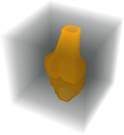 |
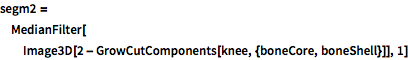
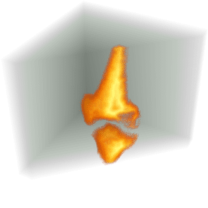
Run the 3D grow-cut-algorithm to refine the segmentation.
| Out[7]= |  |
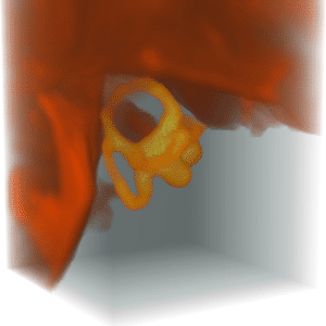
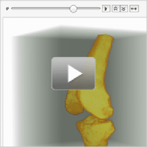
Visualize the segmentation.
| Out[8]= |  |
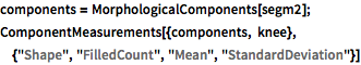
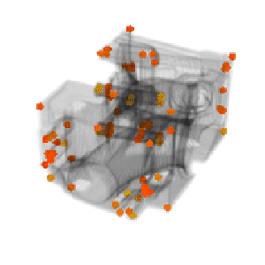
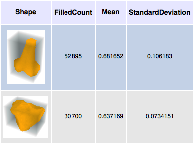
Size and density measurements can be calculated for each segment.
| Out[9]= |  |
| Out[37]//TraditionalForm= |
| |  |