求解带有吸收边界条件的波动方程
求解一维带有吸收边界条件的波动方程.
指定一个带有吸收边界条件的波动方程. 注意诺依曼(Neumann)值是用于  的一阶时间导数的.
In[1]:=
eqn = D[u[t, x], {t, 2}] ==
   D[u[t, x], {x, 2}] +
    NeumannValue[-Derivative[1, 0][u][t, x], x == 0 || x == 1];
指定波动方程的初始条件.
In[2]:=
u0[x_] := Evaluate[D[0.125 Erf[(x - 0.5)/0.125], x]];
ic = {u[0, x] == u0[x], Derivative[1, 0][u][0, x] == 0};
使用有限元方法求解方程.
In[3]:=
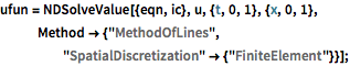
ufun = NDSolveValue[{eqn, ic}, u, {t, 0, 1}, {x, 0, 1},
Method -> {"MethodOfLines",
"SpatialDiscretization" -> {"FiniteElement"}}];可视化带有吸收边界条件的波动方程.
In[4]:=
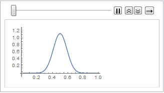
list = Table[
   Plot[ufun[t, x], {x, 0, 1}, PlotRange -> {-0.1, 1.3}], {t, 0, 1,
    0.1}];
ListAnimate[list]