Kleine Schwankungen in einem CO-Molekül modellieren

In einem Experiment schwankt ein CO-Molekül um seine Gleichgewichtslänge mit einer effektiven Federkonstante . Die Schwankungen folgen der Gleichung für harmonische Bewegung. Im Folgenden ist die reduzierte Masse des Moleküls, die natürliche Frequenz, die Entfernung von der Gleichgewichtslage und das plancksche Wirkungsquantum.

In[1]:=

qho = -(\[HBar]^2/(2 m)) Laplacian[u[x], {x}] + (m \[Omega]^2)/ 2 x^2 u[x];

Berechnen Sie die ersten vier Eigenwerte und normalisierten Eigenfunktionen.

In[2]:=

sol = DEigensystem[qho, u[x], {x, -\[Infinity], \[Infinity]}, 4, Assumptions -> \[HBar] > 0 && m > 0 && \[Omega] > 0, Method -> "Normalize"]

Out[2]=

Unter der Annahme, dass sich das Teilchen in einer Überlagerung der vier Einzelzustände befindet, nimmt die Wellenfunktion die Form an.

In[3]:=

\[Psi][x_, t_] = Total[MapThread[1/2 Exp[I E t #1/\[HBar]] #2 &, sol]]

Out[3]=

Berechnen Sie die drei Parameter , und unter Verwendung von Basisgrößen für atomare Masseneinheiten (Femtosekunden und Pikometer), da die resultierenden Werte nahe bei 1 liegen.

In[4]:=

m = QuantityMagnitude[( Entity["Element", "Carbon"][ EntityProperty["Element", "AtomicMass"]] Entity["Element", "Oxygen"][EntityProperty["Element", "AtomicMass"]])/( Entity["Element", "Carbon"][ EntityProperty["Element", "AtomicMass"]] + Entity["Element", "Oxygen"][ EntityProperty["Element", "AtomicMass"]]), "AtomicMassUnits"]

Out[4]=

In[5]:=

\[Omega] = Sqrt[QuantityMagnitude[Quantity[1.86, "Kilonewtons"/"Meters"], "AtomicMassUnit"/"Femtoseconds"^2]/m]

Out[5]=

In[6]:=

\[HBar] = QuantityMagnitude[Quantity[1., "ReducedPlanckConstant"], "AtomicMassUnit"*"Picometers"^2/"Femtoseconds"]

Out[6]=

Die Wahrscheinlichkeitsdichtefunktion der Entferung ist gegeben durch .

In[7]:=

\[Rho][x_, t_] = FullSimplify[ComplexExpand[Conjugate[\[Psi][x, t]] \[Psi][x, t]]]

Out[7]=

Als Wahrscheinlichkeitsfunktion ist das Integral von über den reellen Zahlen 1 für alle .

In[8]:=

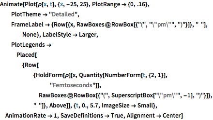
Chop[Integrate[\[Rho][x, t], {x, -\[Infinity], \[Infinity]}]]

Out[8]=

Visualisieren Sie die Wahrscheinlichkeitsdichte im Lauf der Zeit.

In[9]:=

Animate[Plot[\[Rho][x, t], {x, -25, 25}, PlotRange -> {0, .16}, PlotTheme -> "Detailed", FrameLabel -> {Row[{x, RawBoxes@RowBox[{"(", "\"pm\"", ")"}]}, " "], None}, LabelStyle -> Larger, PlotLegends -> Placed[{Row[{HoldForm[\[Rho]][x, Quantity[NumberForm[t, {2, 1}], "Femtoseconds"]], RawBoxes@RowBox[{"(", SuperscriptBox["\"pm\"", -1], ")"}]}, " "]}, Above]], {t, 0., 5.7, ImageSize -> Small}, AnimationRate -> 1, SaveDefinitions -> True, Alignment -> Center]

Animation abspielen

Abspielung unterbrechen