Trouvez la distribution de charge sur une sphère
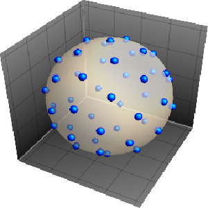
Trouvez les positions qui minimisent le potentiel de Coulomb pour que des particules de même charge puissent se déplacer librement sur une sphère. Voici la répartition des charges à l'équilibre.
Appelez n le nombre de particules.
n = 50;Soit  , les coordonnées cartésiennes de la
  ème particule.
vars = Join[Array[x, n], Array[y, n], Array[z, n]];L'objectif est de minimiser le potentiel de Coulomb.
potential =
  Sum[((x[i] - x[j])^2 + (y[i] - y[j])^2 + (z[i] - z[j])^2)^-(1/
       2), {i, 1, n - 1}, {j, i + 1, n}];
Les particules se trouvant sur une sphère, leurs coordonnées doivent satisfaire à des contraintes de magnitude unitaire.
sphereconstr = Table[x[i]^2 + y[i]^2 + z[i]^2 == 1, {i, 1, n}];Choisissez des points initiaux sur la sphère à l'aide de coordonnées sphériques aléatoires.
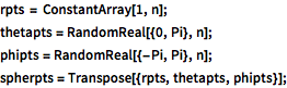
rpts = ConstantArray[1, n];
thetapts = RandomReal[{0, Pi}, n];
phipts = RandomReal[{-Pi, Pi}, n];
spherpts = Transpose[{rpts, thetapts, phipts}];
Transformez les points initiaux en coordonnées cartésiennes.
cartpts = CoordinateTransform["Spherical" -> "Cartesian", spherpts];Réorganisez les points initiaux pour correspondre à la commande de variables.
initpts = Flatten[Transpose[cartpts]];Minimisez le potentiel de Coulomb soumis à la contrainte de la sphère.
sol = FindMinimum[{potential, sphereconstr}, Thread[{vars, initpts}]];Extrayez les positions d'équilibre des particules de la solution.
solpts = Table[{x[i], y[i], z[i]}, {i, 1, n}] /. sol[[2]];Tracez le résultat.
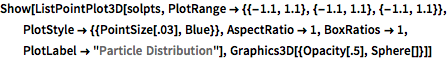
Show[ListPointPlot3D[solpts,
  PlotRange -> {{-1.1, 1.1}, {-1.1, 1.1}, {-1.1, 1.1}},
  PlotStyle -> {{PointSize[.03], Blue}}, AspectRatio -> 1,
  BoxRatios -> 1, PlotLabel -> "Particle Distribution"],
 Graphics3D[{Opacity[.5], Sphere[]}]]