Hidden Markov Processes with Silent States
Hidden Markov processes with silent states are often used with rigid topology of hidden states dynamics, i.e. the transition matrix is sparse, to enable transitions between emitting states that are impossible under the chosen topology. Thanks to the structured transition matrix, hidden Markov models with silent states are frequently easier to estimate than their dense analogs.
Define the initial likelihoods  of the system being in one of six possible unobservable states as well as the matrix
  of the conditional transition probabilities between these states.
| In[1]:= | 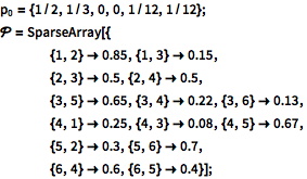 X |
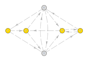
Visualize topology of transitions between hidden states.
| In[2]:= |  X |
| Out[2]= | 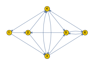 |
Define frequencies of the system emitting a categorical signal for every unobservable state. Emissions are labeled 1 through 6. No emissions are made when the system finds itself in either state 3 or state 4; that is, these states are silent.
| In[3]:= |  X |
Define hidden Markov process that describes observable emissions.
| In[4]:= | X |
Simulate a sequence of emissions.
| In[5]:= | X |
| Out[5]= |
Find the most probable sequence of the system's underlying unobservable states.
| In[6]:= | X |
| Out[6]= |
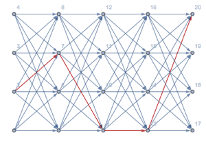
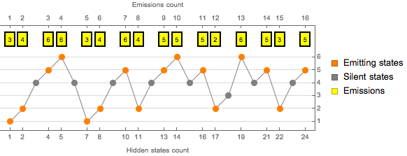
Note that the decoded sequence of states is longer than the sequence of emissions, due to presence of silent states. Visualize the sequence of decoded hidden states.
| In[7]:= | X |
 |
Find the hidden Markov process without hidden states that assigns the same probabilities for all emission sequences.
| In[8]:= | X |
| Out[8]= |  |
Build short sequences of emissions and confirm that both processes assign them equal likelihoods.
| In[9]:= | X |
| In[10]:= | X |
| In[11]:= | X |
| In[12]:= | X |
| Out[12]= |
Generate an ensemble of longer emission sequences and use it to estimate parameters of the hidden Markov process with silent states.
| In[13]:= | X |
| In[14]:= | X |
| Out[14]= |  |
Compare log-likelihoods of emissions.
| In[15]:= | X |
| Out[15]= |
| In[16]:= | X |
| Out[16]= |
