Learn a Parameterization of a Manifold
Learn a parameterization of the manifold along which the input data lies by using an autoencoder, a network with a "bottleneck" layer that learns to reconstruct the original input.
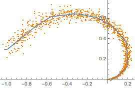
Sample training data from a part of a synthetic two-dimensional manifold.

manifold =
  Table[AngleVector[{x, 0.9 Pi x}] +
    x/20*RandomVariate[NormalDistribution[], 2], {x, 0, 1, 0.001}];
plot = ListPlot[manifold, PlotStyle -> Orange]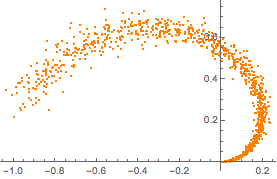
Create a net with a "bottleneck" layer in order to learn a parameterization of the manifold.
net = NetChain[{25, Ramp, 1, 25, Ramp, 2}, "Input" -> 2]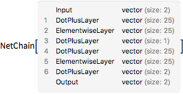
Create a loss network that computes a loss based on the "reconstruction error"—a measure of the degree to which the network can produce an output that is identical to its input.
lossNet =
 NetGraph[{net, MeanSquaredLossLayer[]}, {1 -> 2,
   NetPort["Input"] -> NetPort[2, "Target"]}]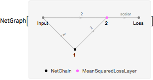
Train the loss network on the manifold and extract the original net from the loss network.
lossNet =
  NetTrain[lossNet, <|"Input" -> manifold|>, BatchSize -> 4096];
trained = NetExtract[lossNet, 1];
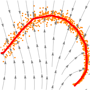
Visualize how the net projects arbitrary points onto the manifold.

{{xmin, xmax}, {ymin, ymax}} = CoordinateBounds[manifold, .2];
Show[plot,
 StreamPlot[
  trained[{x, y}] - {x, y}, {x, xmin, xmax}, {y, ymin, ymax}]]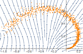
Split the net into an "encoder" and "decoder" network (the encoder parameterizes points using a single scalar value, whereas the decoder reconstructs the point from this parameterization).
decoder = Drop[trained, 3]
encoder = Take[trained, 3]

Color each point in the original manifold by its parameterization under the encoder.
ListPlot[Style[#, Hue[First[0.3 + encoder[#]]/3]] & /@ manifold]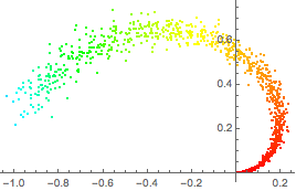
Obtain the range of the parameterization by applying the encoder to the manifold.
{min, max} = MinMax[encoder[manifold]]Show the reconstruction over this range along with the original manifold.
Show[plot, ListLinePlot[Table[decoder[x], {x, min, max, .01}]]]