基本解を使って波動方程式を解く

一空間次元における波動方程式を定義する．

In[1]:=

waveOperator = \!\( \*SubscriptBox[\(\[PartialD]\), \({t, 2}\)]\(u[x, t]\)\) - \!\( \*SubscriptBox[\(\[PartialD]\), \({x, 2}\)]\(u[x, t]\)\);

GreenFunctionを使って，その基本解を得る．

In[2]:=

gf[x_, t_, y_, s_] = GreenFunction[waveOperator, u[x, t], {x, -\[Infinity], \[Infinity]}, t, {y, s}]

Out[2]=

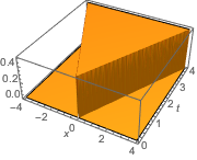
基本解をプロットする．

In[3]:=

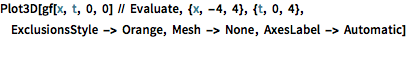
Plot3D[gf[x, t, 0, 0] // Evaluate, {x, -4, 4}, {t, 0, 4}, ExclusionsStyle -> Orange, Mesh -> None, AxesLabel -> Automatic]

Out[3]=

強制関数を定義する．

In[4]:=

f[y_, s_] := Cos[y] E^(-s)

たたみ込み積分 を評価することによって，この強制項を持つ波動方程式を解く．

In[5]:=

sol = Integrate[ gf[x, t, y, s] f[y, s], {y, -\[Infinity], \[Infinity]}, {s, 0, \[Infinity]}, Assumptions -> t > 0 && Im[x] == 0] // FullSimplify

Out[5]=

斉時初期条件を含む結果をDSolveValueを使って得る．

In[6]:=

initialc = {u[x, 0] == 0, Derivative[0, 1][u][x, 0] == 0};

In[7]:=

DSolveValue[{waveOperator == f[x, t], initialc}, u[x, t], {x, t}]

Out[7]=

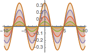
解によって生成された定常波を可視化する．

In[8]:=

Plot[Table[sol, {t, 0, 1, 0.2}] // Evaluate, {x, -10, 10}, Filling -> Axis]

Out[8]=