Model a Hanging Chain
Find the position with minimal potential energy of a chain or cable of length  suspended between two points.
Set parameter values for the length of the chain  , the left-end height
  , and the right-end height
  .
.
L = 4; a = 1; b = 3; Let  be the height of the chain as a function of horizontal position, with
  .
.
xf = 1; nh = 201; h := xf/nh;Set up variables for the height of the chain  .
.
varsy = Array[y, nh + 1, {0, nh}];Denote the slope at position  by
by  and set up variables for it.
varsm = Array[m, nh + 1, {0, nh}];Denote the partial potential energy from  to
to  by
by 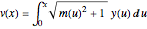 .
.
varsv = Array[v, nh + 1, {0, nh}];Denote the length of the chain at position  by
by  and set up variables for it.
varss = Array[s, nh + 1, {0, nh}];Join all variables.
vars = Join[varsm, varsy, varsv, varss];The objective is to minimize the total potential energy  .
.
objfn = v[nh];Here are the boundary value constraints from the geometry.
bndcons = {y[0] == a, y[nh] == b, v[0] == 0, s[0] == 0, s[nh] == L}; Discretize the ODEs:  ,
,  ,
,  .
.
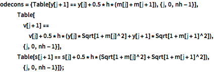
odecons = {Table[
    y[j + 1] == y[j] + 0.5*h*(m[j] + m[j + 1]), {j, 0, nh - 1}],
   Table[v[j + 1] ==
     v[j] + 0.5*
       h*(y[j]*Sqrt[1 + m[j]^2] + y[j + 1]*Sqrt[1 + m[j + 1]^2]), {j,
     0, nh - 1}],
   Table[s[j + 1] ==
     s[j] + 0.5*h*(Sqrt[1 + m[j]^2] + Sqrt[1 + m[j + 1]^2]), {j, 0,
     nh - 1}]};
Choose initial points for the variables.
tmin = If[b > a, 0.25 , 0.75]; init =
 Join[Table[4*Abs[b - a]*((k/nh) - tmin), {k, 0, nh}],
  Table[4*Abs[b - a]*(k/nh)*(0.5*(k/nh) - tmin) + a, {k, 0, nh}],
  Table[(4*Abs[b - a]*(k/nh)*(0.5*(k/nh) - tmin) + a)*4*
    Abs[b - a]*((k/nh) - tmin), {k, 0, nh}],
  Table[4*Abs[b - a]*((k/nh) - tmin), {k, 0, nh}]];
Minimize the total potential energy, subject to the constraints.
sol = FindMinimum[{objfn, Join[bndcons, odecons]},
   Thread[{vars, init}]];
Extract the solution points.
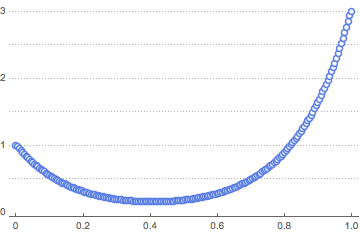
solpts = Table[{i h, y[i] /. sol[[2]]}, {i, 0, nh}];Plot the position of the chain with minimal potential energy.
ListPlot[solpts, ImageSize -> Medium, PlotTheme -> "Marketing"]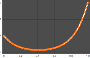
Use FindFit to fit the result to the catenary curve.
catenary[t_] = c1 + (1/c2) Cosh[c2 (t - c3)];fitsol = FindFit[solpts, catenary[t], {c1, c2, c3}, {t}]Plot the solution points together with the catenary curve.
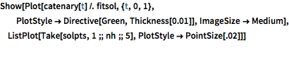
Show[Plot[catenary[t] /. fitsol, {t, 0, 1},
  PlotStyle -> Directive[Green, Thickness[0.01]],
  ImageSize -> Medium],
 ListPlot[Take[solpts, 1 ;; nh ;; 5], PlotStyle -> PointSize[.02]]]