Compute Expectation of Autoregressive Moving-Average Process from Its Definition
This example explores an ARMA process with initial values. It constructs process values in terms of the sequence of innovations and uses enhanced support of random processes in Expectation to compute the mean and covariance of the process slices. Furthermore, stationary time series process is reinterpreted as time series process with random initial values.
Define autoregressive moving-average process values via its defining relation as a function of driving white noise process values  .
.
| In[1]:= | X |
| Out[1]= |
Process values for ARMA(2,1) process.
| In[2]:= | X |
Compute mean of process values  for
for  , given past process values, and given zero values of innovations in the past.
| In[3]:= | X |
| In[4]:= | X |
| Out[4]= |  |
Compare to the values of the process mean function.
| In[5]:= | X |
| Out[5]= |
Use Expectation to compute covariance function of process values under the same conditions.
| In[6]:= |  X |
| Out[6]//Short= | |
 | |
Covariance function for a particular value of process parameters.
| In[7]:= | X |
| Out[7]//MatrixForm= | |
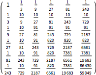 | |
Compare computed covariance matrix to values of CovarianceFunction.
| In[8]:= | X |
| Out[8]= |
Compute mean and covariance of process values assuming a Gaussian joint distribution for past values and past innovations.
| In[9]:= | X |
| In[10]:= | X |
| In[11]:= |  X |
| Out[11]= |  |
| In[12]:= |  X |
| Out[12]//Short= | |
 | |
Weak stationarity condition implies that the mean values should be equal and the covariance matrix values across subdiagonals should be the same. This determines parameters of the joint distribution of past values.
| In[13]:= |  X |
| Out[13]= |  |
Compare to the covariance function of weakly stationary ARMA(2,1) process.
| In[14]:= |  X |
| Out[14]= |
