Log Returns of Stock Prices

Stock prices modeled with geometric Brownian motion (in the classical Black–Scholes model) are assumed to be normally distributed in their log returns. Here, this assumption is examined with the stock prices of five companies: Google, Microsoft, Facebook, Apple, and Intel.

Retrieve the stock prices in 2015 with FinancialData.

In[1]:=

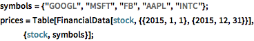
symbols = {"GOOGL", "MSFT", "FB", "AAPL", "INTC"}; prices = Table[ FinancialData[stock, {{2015, 1, 1}, {2015, 12, 31}}], {stock, symbols}];

Compute the log returns.

In[2]:=

logreturn = Minus[Differences[Log[prices[[All, All, 2]]], {0, 1}]];

Filter the log returns with an ARCHProcess of order 1.

In[3]:=

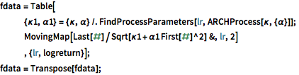
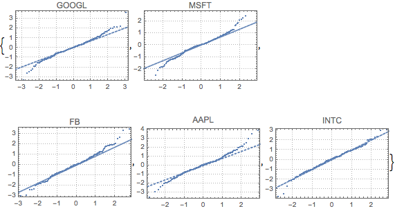
fdata = Table[ {\[Kappa]1, \[Alpha]1} = {\[Kappa], \[Alpha]} /. FindProcessParameters[lr, ARCHProcess[\[Kappa], {\[Alpha]}]]; MovingMap[Last[#]/Sqrt[\[Kappa]1 + \[Alpha]1 First[#]^2] &, lr, 2] , {lr, logreturn}]; fdata = Transpose[fdata];

Compare the filtered data from each stock to the normal distribution with QuantilePlot. For all five companies, the tails deviate from normal.

In[4]:=

MapThread[ QuantilePlot[#1, PlotLabel -> #2, PlotTheme -> "Detailed"] &, {Transpose[fdata], symbols}]

Out[4]=

Perform a multivariate normality test with BaringhausHenzeTest (BHEP). The normality assumption is clearly rejected.

In[5]:=

htd = BaringhausHenzeTest[fdata, "HypothesisTestData"];

In[6]:=

htd["TestDataTable"]

Out[6]=

In[7]:=

htd["ShortTestConclusion"]

Out[7]=

Fit the filtered data with MultinormalDistribution and MultivariateTDistribution.

In[8]:=

multiN = EstimatedDistribution[fdata, MultinormalDistribution[Array[x, 5], Array[s, {5, 5}]]]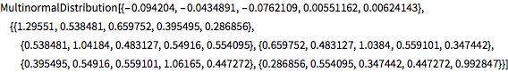

Out[8]=

In[9]:=

multiT = EstimatedDistribution[fdata, MultivariateTDistribution[Array[x, 5], Array[s, {5, 5}], nu]]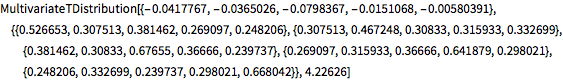

Out[9]=

Compute the AIC for the two distributions. The model of MultivariateTDistribution has a smaller value.

In[10]:=

aic[k_, dist_, data_] := 2 k - 2 LogLikelihood[dist, data]

In[11]:=

aic[5 + 15, multiN, fdata]

Out[11]=

In[12]:=

aic[5 + 15 + 1, multiT, fdata]

Out[12]=